
JAX-in-the-Box: Unboxing Stateful Training with Flax NNX and Orbax
March 2026
Background: The Evolution of JAX
Born from years of scaling TensorFlow and engineered to meet the demands of modern, highly flexible AI research, JAX has become Google’s flagship platform for high-performance numerical computing. Today, JAX powers the vast majority of Google’s breakthrough research and generative AI initiatives, including AlphaFold, Gemini, and Gemma.
Architecturally, JAX achieves unrivaled hardware portability compared to other legacy deep learning frameworks. By leveraging the XLA (Accelerated Linear Algebra) compiler as its unified backend, JAX can compile identical Python code into optimized machine instructions across different hardware platforms.
For years, however, choosing between PyTorch and JAX required accepting a philosophical tradeoff: PyTorch offered developers intuitive, object-oriented state management (via torch.nn.Module), while JAX strictly demanded functional purity. To manage neural network weights in traditional JAX frameworks, developers had to manually extract, pass, and return dictionary states (pytrees) through every single computational function.
That paradigm has officially shifted. With the stabilization of Flax NNX, JAX introduced a native stateful, object-oriented API. It delivers the modular feel of PyTorch while preserving the raw, composable functional transformations that make JAX unique.
In this post, we will walk through an end-to-end training and checkpointing pipeline for a simple Multi-Layer Perceptron (MLP) using Flax NNX and Orbax. We will also briefly touch on how this modern stack achieves seamless hardware portability across CPUs, GPUs, and TPUs without changing a single line of code, a capability you can verify yourself using the free accelerator tiers in Google Colab. An interactive Notebook version of this blog is available for you to run it on your local machine or in Google Colab.
End-to-End Implementation: Building an MLP Pipeline
In the following section, we will build a self-contained AI stack step-by-step:
- Initialize an MLP with a hidden layer and an output layer.
- Setup and stream synthetic batches using two distinct dataloading paradigms.
- Train the model using an encapsulated JIT-compiled loop while tracking loss convergence.
- Export and restore the optimized state safely using Orbax.
Environment Setup and Core Imports
Before writing model logic, we pull in the foundational libraries of our ecosystem: JAX for array operations, Optax for optimization algorithms, Flax NNX for stateful neural network blocks, and Orbax for high-performance checkpointing.
import os
import shutil
from pathlib import Path
import numpy as np
import matplotlib.pyplot as plt
from tqdm.notebook import tqdm

import torch
from torch.utils.data import Dataset, DataLoader

import jax
import jax.numpy as jnp
import grain.python as grain
from flax import nnx
import optax
import orbax.checkpoint as ocp
Defining the Stateful Model Architecture
In classic Flax (Linen), variables and parameters were kept completely separate from the architecture definition. In Flax.nnx, parameters live directly inside our custom objects (e.g., self.dense_layer_1). NNX uses dynamic proxy objects under the hood to automatically discover child modules and their respective weights.
# Create a stateful MLP by inheriting from the native nnx.Module
class MySimpleMlp(nnx.Module):
    def __init__(self, din: int, dout: int, rngs: nnx.Rngs):
        # Parameters (weights/biases) are encapsulated inside these submodules automatically
        self.dense_layer_1 = nnx.Linear(din, 5, rngs=rngs)
        self.dense_layer_2 = nnx.Linear(5, dout, rngs=rngs)

    def __call__(self, x) -> jnp.ndarray:
        # Define the forward pass using clear, standard imperative execution
        x = self.dense_layer_1(x)
        x = nnx.relu(x)
        x = self.dense_layer_2(x)
        return x
Functional Train Step and In-Place JIT Mutation
JAX demands functional purity, meaning side effects like in-place variable mutation are strictly forbidden inside a @jax.jit compiled function.
NNX solves this elegantly via nnx.jit. When we pass an nnx.Module or nnx.Optimizer into an NNX-compiled function, the framework automatically executes an nnx.split() right before entering the JIT boundary. This breaks our stateful object down into a static structure graph and a dynamic array pytree. Once the function finishes running, it automatically merges them back together, allowing us to use intuitive, object-oriented patterns like optimizer_arg.update(model_arg, grads) smoothly:
# The nnx.jit decorator safely manages stateful objects crossing the JIT boundary
@nnx.jit
def train_step(model_arg: nnx.Module, optimizer_arg: nnx.Optimizer,
               x_batch: jnp.ndarray, y_batch: jnp.ndarray) -> jnp.ndarray:

    # Internal pure function mapping input parameters to a scalar loss
    def loss_fn_for_grad(model_in_grad_fn: nnx.Module) -> float:
        y_pred = model_in_grad_fn(x_batch)
        return jnp.mean((y_batch - y_pred) ** 2)

    # nnx.value_and_grad cleanly extracts the dynamic pytree values and their gradients
    loss_value, grads = nnx.value_and_grad(loss_fn_for_grad)(model_arg)

    # Mutates optimizer state in-place; NNX abstracts this side effect away safely
    optimizer_arg.update(model_arg, grads)
    return loss_value
Setting up a Dataset and DataLoader Pipeline
To feed batches of data into our model seamlessly during training, we need a robust data pipeline. We have two primary paths to achieve this: leveraging the familiar PyTorch framework (restricted purely to the host CPU) or adopting Google's new JAX-native data loading engine, Grain.
Here, we will break down both approaches and show how easily they integrate into our Flax NNX training loop.
Approach A: The PyTorch Host-Side Loader
It is a common concern among developers that introducing PyTorch utilities into a JAX project might trigger hardware allocation conflicts or portability bugs. However, PyTorch’s data loading pipeline is completely decoupled from its GPU execution engine. When we configure a PyTorch DataLoader, it operates strictly on the host (CPU), utilizing standard Python multiprocessing to fetch, shuffle, and structure our samples. Because it leaves the data resident on the CPU without touching accelerator drivers, it is 100% compatible with the JAX ecosystem and will not interfere with JAX’s device management on GPUs or TPUs.
Important JAX Integration Note: To make PyTorch fully compatible with JAX, we intercept batch formation using a custom
numpy_collatefunction. This overrides PyTorch's default tensor behavior, ensuring that data batches are yielded as native NumPy arrays rather thantorch.Tensorobjects. JAX instantly digests raw NumPy arrays inside an@nnx.jitfunction and transparently routes them to our active hardware accelerator.
# Set a CPU-side seed for reproducible dummy data generation
torch.manual_seed(123)

class MySimpleDataset(Dataset):
    def __init__(self, num_examples: int, din: int, dout: int):
        # Generate raw synthetic data features and labels on the CPU host
        self.x_data = torch.randn(num_examples, din)
        self.y_data = torch.randn(num_examples, dout)

    def __len__(self) -> int:
        return self.x_data.shape[0]

    def __getitem__(self, idx):
        return self.x_data[idx], self.y_data[idx]

def numpy_collate(batch):
    """Intercepts the batch to collate samples into pure NumPy arrays."""
    transposed = zip(*batch)
    return [np.array(samples) for samples in transposed]

def create_pytorch_loader(num_examples: int, din: int, dout: int,
                          batch_size: int = 8, shuffle: bool = True) -> DataLoader:
    """Factory function initializing our host-safe PyTorch data stream."""
    dataset = MySimpleDataset(num_examples=num_examples, din=din, dout=dout)
    return DataLoader(
        dataset=dataset,
        batch_size=batch_size,
        shuffle=shuffle,
        num_workers=0,            # Keep execution on the main host thread for simplicity
        collate_fn=numpy_collate, # Map tensors out, map NumPy arrays in
        drop_last=True
    )
Approach B: Google Grain (The JAX-Native Alternative)
If we want to maintain a pure, single-ecosystem software stack, Google’s Grain is the optimal choice. Grain is a modern open-source data loader engineered from the ground up specifically for JAX environments.
Grain is incredibly lightweight, built purely around Python/JAX conventions, and introduces production-grade advantages like deterministic checkpointing. If a multi-day training job unexpectedly crashes mid-run, Grain’s internal state can be checkpointed alongside our model weights. When restored, the loader knows exactly how to resume streaming from the precise index slice where it left off, avoiding redundant data processing.
The Tradeoff: Because Grain is a newer addition to the AI landscape, it features a smaller community footprint and fewer pre-built text or vision transformation libraries compared to PyTorch.
def create_grain_loader(num_examples: int, din: int, dout: int, batch_size: int = 8):
    """Creates a deterministic, native JAX data loader using Google Grain."""
    # Generate standard host arrays using NumPy
    rng = np.random.default_rng(123)
    x_data = rng.standard_normal(size=(num_examples, din)).astype(np.float32)
    y_data = rng.standard_normal(size=(num_examples, dout)).astype(np.float32)

    # Wrap the data inside an indexable Grain MapDataset source
    data_source = grain.MapDataset.source(list(zip(x_data, y_data)))

    # Construct a pipeline with deterministic batch transformations
    pipeline = data_source.map(lambda item: (item[0], item[1]))
    pipeline = pipeline.batch(batch_size=batch_size, drop_remainder=True)

    return pipeline
Setting up Data Batch Streams
JAX handles randomness via explicit, deterministic pseudo-random number generator (PRNG) state keys rather than global hidden seeds. In this step, we safely split our source entropy into dedicated keys for network weight initialization, followed by setting up our uniform dataset boundaries.
# Initialize the functional random state using a base seed
main_key = jax.random.PRNGKey(42)
# Split the key: one for current parameter initialization, one reserved for future entropy
model_key, main_key = jax.random.split(main_key, 2)

# Establish model dimensions, batch size
num_examples = 1000
batch_size = 16
din = 20
dout = 2

# Instantiate both data streaming pipelines
# The PyTorch loader fetches data on the host CPU and yields batches via our NumPy collator
pytorch_loader = create_pytorch_loader(num_examples=num_examples, din=din, dout=dout, batch_size=batch_size)

# The Grain loader creates a native, deterministic JAX-friendly data stream on the host CPU
grain_loader = create_grain_loader(num_examples=num_examples, din=din, dout=dout, batch_size=batch_size)
Executing the Optimization Loop
With our compiled training step set up, we define a training loop across an arbitrary number of epochs. Because train_step is optimized by XLA, subsequent iterations bypass Python overhead entirely, executing faster.
def train_loop(model: nnx.Module, optimizer: nnx.Optimizer,
               data_loader, num_epochs: int) -> list[float]:
    """
    Executes a standard training loop over either a PyTorch DataLoader
    or a Google Grain MapDataset pipeline with real-time tqdm metrics.
    """
    epoch_losses = []

    # Assign the tqdm progress bar to a variable ('pbar')
    pbar = tqdm(range(num_epochs), desc="Training Progress")

    for epoch in pbar:
        running_epoch_loss = 0.0
        total_batches = 0

        # Check if it's a Grain pipeline and extract its underlying iterator.
        # This converts a lazy Grain pipeline into a clean, sliceable batch generator.
        if hasattr(data_loader, "as_numpy_iterator"):
            batch_stream = data_loader.as_numpy_iterator()
        else:
            batch_stream = data_loader # Default fallback for PyTorch DataLoader

        # Stream batches out of our host-side pipeline
        for x_batch, y_batch in batch_stream:

            loss_value = train_step(model, optimizer, x_batch, y_batch)

            # Cast the JAX array to a standard Python float
            # to break the tracking chain and prevent device memory bloat
            running_epoch_loss += float(loss_value)
            total_batches += 1

        # Safely compute the average for the current epoch
        if total_batches > 0:
            average_epoch_loss = running_epoch_loss / total_batches
            epoch_losses.append(average_epoch_loss)

            # Update the progress bar postfix with the latest calculated loss
            pbar.set_postfix(loss=f"{average_epoch_loss:.4f}")
        else:
            epoch_losses.append(0.0)

    return epoch_losses
Execution A: Training Loop with PyTorch Batch Loader
# Instantiate the model architecture
model_rng = nnx.Rngs(params=model_key)
my_model = MySimpleMlp(din, dout, rngs=model_rng)

# Bind the model parameters to an Optax-backed stateful optimizer
optax_tx = optax.adam(learning_rate=0.001)
# wrt=nnx.Param instructs the optimizer to track specifically the trainable Param variables
my_optimizer = nnx.Optimizer(my_model, optax_tx, wrt=nnx.Param)

num_epochs = 100
loss_pytorch = train_loop(my_model, my_optimizer, pytorch_loader, num_epochs)
Execution B: Training Loop with Grain Batch Loader
# Instantiate an identical fresh model architecture
model_rng = nnx.Rngs(params=model_key)
my_model = MySimpleMlp(din, dout, rngs=model_rng)

# Bind the model parameters to an Optax-backed stateful optimizer
optax_tx = optax.adam(learning_rate=0.001)
my_optimizer = nnx.Optimizer(my_model, optax_tx, wrt=nnx.Param)

num_epochs = 100
loss_grain = train_loop(my_model, my_optimizer, grain_loader, num_epochs)
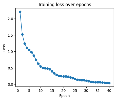
Visualizing Loss Convergence Over Epochs
fig, ax = plt.subplots(figsize=(5, 4))
ax.plot(range(1, num_epochs+1), loss_pytorch, '.-', color='blue', label='PyTorch Dataloader')
ax.plot(range(1, num_epochs+1), loss_grain, '.-', color='red', label='Grain Dataloader')
ax.set_title("Training Loss Over Epochs")
ax.set_xlabel("Epoch")
ax.set_ylabel("Loss")
plt.legend()
plt.show()
Visualizing Internals: Extracting Weights and Biases
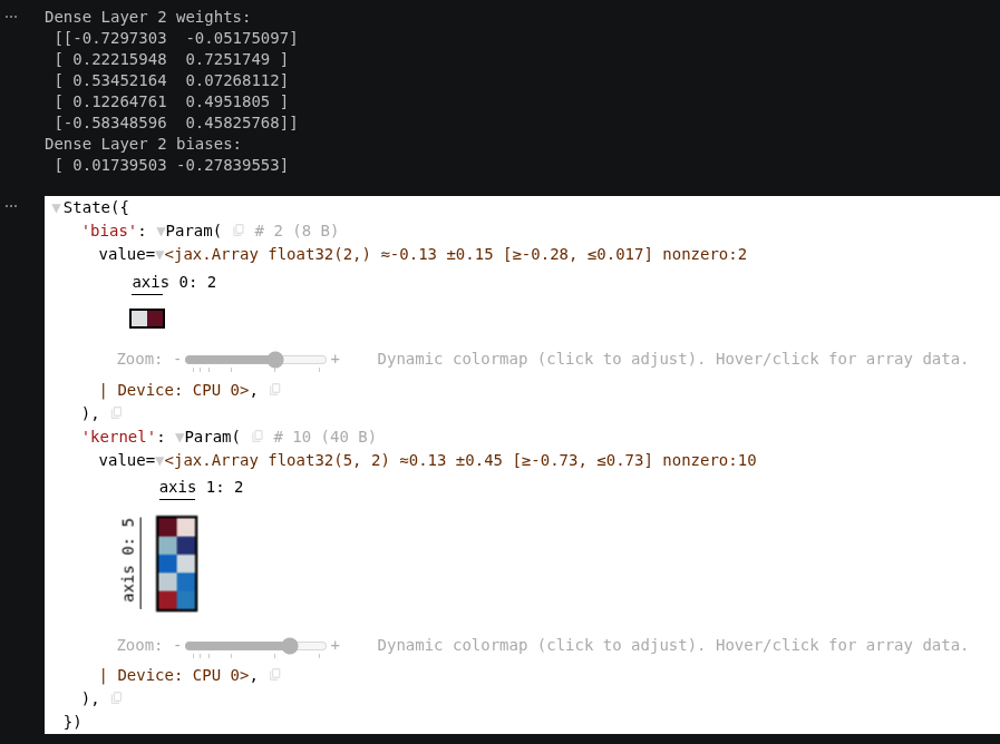
Flax NNX variables implement slicing semantics to expose raw tracking data. The ellipsis syntax [...] is used to select all elements across all array dimensions without needing a deprecated .value property.
# 'nnx.split' separates the static architecture graph from the dynamic array PyTree
_, model_state = nnx.split(my_model)

# Accessing the underlying layer parameters directly from the state leaves via [...]
layer_2_weights = model_state.dense_layer_2.kernel[...]
layer_2_biases  = model_state.dense_layer_2.bias[...]

print("Dense Layer 2 weights:\n", layer_2_weights)
print("Dense Layer 2 biases:\n", layer_2_biases)

# Another way to browse state PyTree layout structurally
nnx.display(model_state.dense_layer_2)
Initializing Production-Grade Checkpointing via Orbax
When saving model weights using orbax.checkpoint, we will encounter serialization failures if we pass a relative path (like ../model-checkpoints). Orbax relies heavily on Google's TensorStore engine to coordinate asynchronous, multi-threaded array caching. TensorStore requires strict absolute paths (Path.resolve()) to ensure no file shards are misplaced during intensive write routines.
Before saving, we extract the underlying raw dictionary data weights out of our stateful classes using nnx.split(). This creates a serialization-ready bundle containing pure arrays that TensorStore can effortlessly stream onto the disk.
# Convert storage folder into a strict absolute path to satisfy TensorStore
checkpoint_dir = Path.cwd().parent.resolve().joinpath('model-checkpoints')
if checkpoint_dir.exists():
    shutil.rmtree(checkpoint_dir) # Clean out any existing checkpoints from prior runs

# Initialize manager configurations
current_step = num_epochs
mngr_options = ocp.CheckpointManagerOptions(save_interval_steps=1, max_to_keep=1)
mngr = ocp.CheckpointManager(checkpoint_dir, options=mngr_options)

# Strip away object metadata, leaving behind pure JAX dictionary states (pytrees)
_, model_state_to_save = nnx.split(my_model)
_, optimizer_state_to_save = nnx.split(my_optimizer)

# Construct a dictionary containing the pure states
save_bundle = {
    'model': model_state_to_save,
    'optimizer': optimizer_state_to_save,
    'current_step': current_step
}

# Stream out saved objects asynchronously and block until completion
mngr.save(current_step, args=ocp.args.StandardSave(save_bundle))
mngr.wait_until_finished()
print(f"Model successfully checkpointed to absolute path: {checkpoint_dir}")
Restoring Checkpoint State
To restore a checkpoint, we initialize a fresh instance of our model and Optax transform. The new model, restored_model, is instantiated with a completely different PRNG key to demonstrate that state overwrite works correctly. We then use checkpoint_manager.restore() with ocp.args.StandardRestore() to pull the bundled dictionaries back into host memory.
We then update the internal state of our target containers in-place using the native utility nnx.update(). Finally, we assert that the restored matrices perfectly mirror our pre-saved weights.
# Initialize a new model instance with a fresh, distinct RNG key
restore_key, main_key = jax.random.split(main_key, 2)
restored_model_rng = nnx.Rngs(params=restore_key)
restored_model = MySimpleMlp(din=din, dout=dout, rngs=restored_model_rng)
restored_optax_tx = optax.adam(learning_rate=0.1)

# Fetch the latest available checkpoint from disk via Orbax
loaded_bundle = None
if mngr:
    latest_step = mngr.latest_step()
    if latest_step is not None:
        # standard_restore reads the structured pytree files directly into memory
        loaded_bundle = mngr.restore(latest_step, args=ocp.args.StandardRestore(save_bundle))
        print(f"Checkpoint was restored from step {latest_step}")
    else:
        print("No checkpoint was found to restore.")
else:
    print("Checkpointing manager not initialized for restore.")

# Apply the loaded states to our empty container instances
if loaded_bundle and restored_model:
    # nnx.update mutates the model in-place, filling its parameters with the loaded arrays
    nnx.update(restored_model, loaded_bundle['model'])
    print("Restored model's state applied.")

    # Initialize the optimizer *after* updating the model so it tracks the correct initial weights
    restored_optimizer = nnx.Optimizer(restored_model, restored_optax_tx, wrt=nnx.Param)
    nnx.update(restored_optimizer, loaded_bundle['optimizer'])
    print("Restored optimizer's state applied.")
else:
    print("Loaded_bundle or restored_model is None, cannot apply states.")

# Verify Model Array Equality
original_kernel = save_bundle['model'].dense_layer_1.kernel[...]
_, restored_model_state = nnx.split(restored_model) # Split into a pure pytree to extract arrays
restored_kernel = restored_model_state.dense_layer_1.kernel[...]

assert jnp.array_equal(original_kernel, restored_kernel), "Model states differ!"
print('Model state restore verified successfully.')

# Verify Optimizer Array Equality
# Extracting Adam's moving average (mu) directly from Optax's internal tracking dictionary
original_opt_state_adam_mu_kernel = save_bundle['optimizer'].opt_state[0].mu['dense_layer_1']['kernel'][...]
restored_opt_state_adam_mu_kernel = restored_optimizer.opt_state[0].mu['dense_layer_1']['kernel'][...]

assert jnp.array_equal(original_opt_state_adam_mu_kernel, restored_opt_state_adam_mu_kernel), \
                       "Optimizer Adam mu for kernel differs!"
print("Optimizer state (sample mu) restore verified successfully.")

Clean Up and Resource Teardown
Once training and validation are complete, it is best practice to properly close active file streams and manage our persistent storage. Leaving managers open can lock files, and discarding intermediate debugging shards keeps our storage volume clean.
# 1. Gracefully shut down the checkpoint manager to flush any remaining async writes
if mngr:
    mngr.close()
    print("Checkpoint manager closed successfully.")

# 2. Optional: Clean up and delete the checkpoint directory from disk if no longer needed
if checkpoint_dir and checkpoint_dir.exists():
    shutil.rmtree(checkpoint_dir)
    print(f"Cleaned up persistent checkpoint directory at: {checkpoint_dir}")
Hardware Portability: Zero Code Adjustments from CPU to TPU
One of the strengths of this specific JAX/Flax AI stack is its absolute hardware portability.
In frameworks like PyTorch, transitioning a model from a local testing laptop (CPU) to a cloud cluster (GPU or TPU) requires manual device context handling, such as scattering calls like .to('cuda') or .to(device) throughout our model definition and data loading routines.
PyTorch Approach:   [CPU Data] -> .to('cuda') -> [GPU Processing]
JAX/NNX Approach:   [Unified Arrays] -> Automatic JIT Virtual Device Allocation
JAX handles this completely differently through its XLA compiler backend:
Transparent Array Allocation
JAX arrays (jnp.ndarray) are fundamentally device-agnostic abstractions. When we execute JAX code, the arrays are automatically placed on our system's primary default accelerator. If we have a discrete GPU available, JAX initializes our parameters directly inside GPU VRAM; if we are running on a Google Cloud TPU node, they are routed to TPU HBM memory.
The Compiling Layer (@nnx.jit)
The @nnx.jit decorator acts as a high-performance wrapper around jax.jit. Rather than interpreting Python line-by-line, XLA acts as an optimizing compiler. It fuses consecutive mathematical steps (like our Linear layers and relu activation) into unified, hardware-optimized kernel operations tailored specifically for the target accelerator architecture.
Because XLA abstracts the underlying instruction set, the exact same machine learning pipeline scales seamlessly from single-core CPU testing up to massive TPU-pod configurations with zero architectural changes required.