PyTorch Implementation of Skip-gram with Negative Sampling

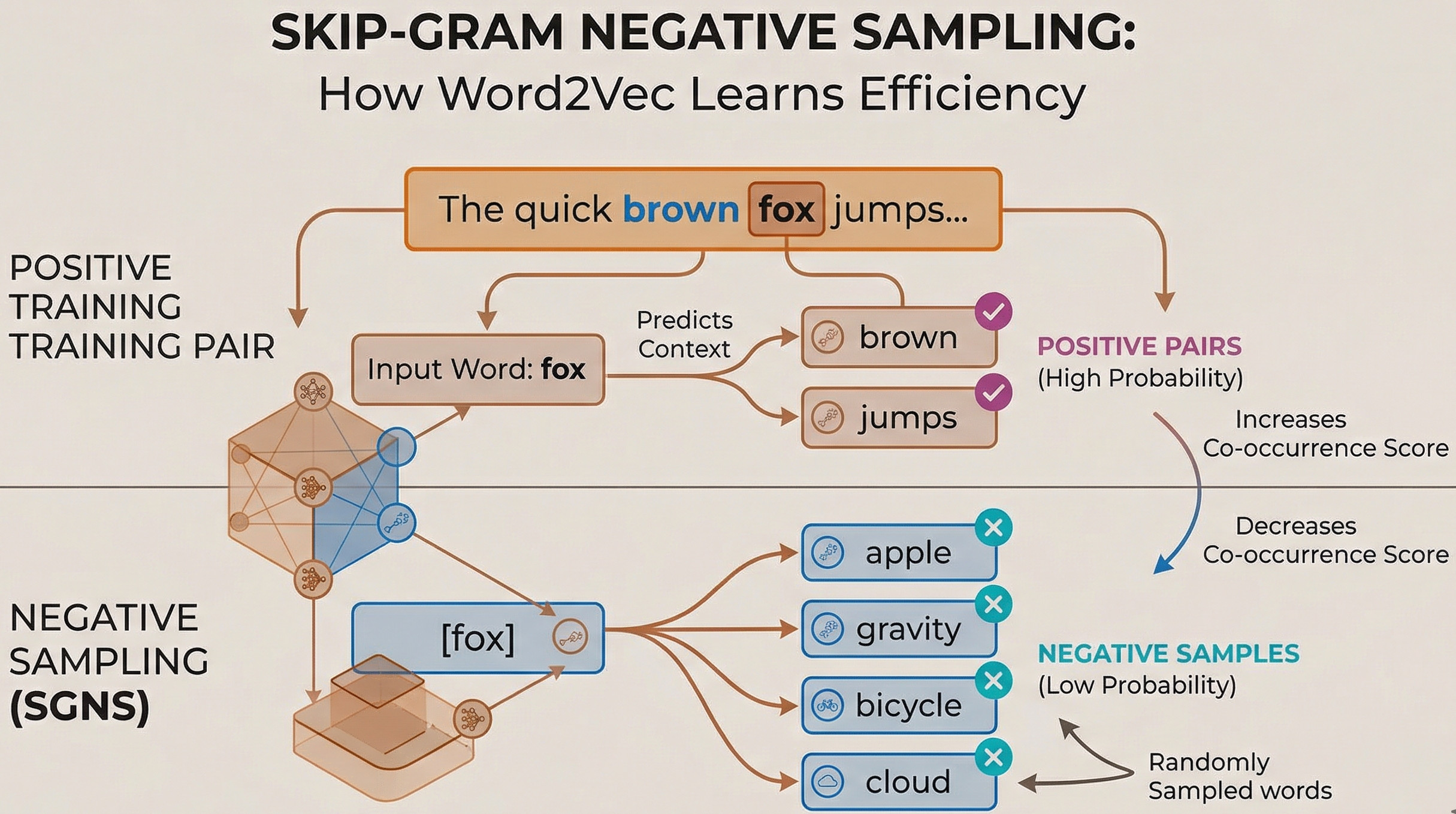
Note: For in-depth technical details and hands-on experience, you can access the interactive Jupyter Notebook version of this tutorial.

The Negative Sampling Architecture

To implement the Skip-gram Word2Vec model with Negative Sampling, we pivot from the standard "predict a neighbor word" Softmax approach toward a high-speed Binary Classification task. Softmax is computationally expensive for large vocabularies; instead, our model takes two inputs—a Context word and a Target word—and predicts whether they are true neighbors ($1$) or a random pair ($0$).

The Training & Deployment Workflow

The following steps outline the end-to-end process for training the model and preserving the learned embeddings:

1. Prepare and Load the Dataset: Tokenize the corpus and generate (context, positive target, negative samples) triplets using a sliding window.
2. Define the Model: Implement a dual-embedding architecture (Context matrix $E$ and Parameter matrix $\theta$) that uses a dot product to measure word similarity.
3. Define the Loss Objective: Use the Negative Sampling loss function, combining the log-sigmoids of positive and negative scores.
4. Train the Model: Iterate through the dataset, using backpropagation to adjust vectors until words with similar meanings cluster together.
5. Extract and Save Weights: Isolate the trained Matrix $E$ and save it, discarding the temporary classification parameters.
6. Load for Inference: Re-initialize a standalone embedding layer with the saved weights to perform similarity searches.

Preparing and Loading the Dataset

To train a model using Negative Sampling, we must structure our data into batches that contrast real word pairings with random noise. This requires a custom Dataset class to manage context-target pairing and a DataLoader to handle batching and shuffling. Note that we pass numerical indices mapped from our vocabulary, not raw text.

Our custom Word2VecDataset class generates a training triplet for every word:

1. Context: The index of the current "center" word.
2. Positive Target: The index of a word found within a local sliding window (e.g., $\pm 2$ words).
3. Negative Targets: A set of $k$ random indices from the vocabulary that are not the positive target.

Key Technical Implementation Notes

• Memory Efficiency & Regularization: We generate negatives dynamically inside __getitem__. This avoids storing a massive dataset on disk and ensures the model sees different random noise in every epoch, acting as a form of regularization.
• Seamless Batching: The PyTorch DataLoader automatically stacks these triplets into tensors. For a batch_size of $64$ and $k=5$, the negative target tensor becomes $(64, 5)$, aligning perfectly with the Batch Matrix Multiplication (torch.bmm) in our model.

The Role of the __getitem__ Method

This "magic method" is a placeholder in the base torch.utils.data.Dataset. We define it in our subclass so the DataLoader knows how to fetch a specific triplet. Once defined, we can use square bracket notation:

dataset = Word2VecDataset(data, vocab_size)
first_sample = dataset[0] # Triggers dataset.__getitem__(0)

Now, we are ready to implement the class:

import torch
from torch.utils.data import Dataset
import random
import numpy as np

class Word2VecDataset(Dataset):
    """A PyTorch Dataset for Skip-gram word2vec with Negative Sampling."""

    def __init__(self, data, vocab_size, window_size=2, k=5, heuristic_sampling=True):
        self.vocab_size = vocab_size
        self.k = k
        self.pairs = []
        self.heuristic = heuristic_sampling

        # 1. Generate positive pairs by sliding a window over each sequence
        for sequence in data:
            for i, context_word in enumerate(sequence):
                start = max(0, i - window_size)
                end = min(len(sequence), i + window_size + 1)

                for j in range(start, end):
                    if i == j: 
                        continue 
                    self.pairs.append((context_word, sequence[j]))

        # 2. Setup Negative Sampling Distribution (3/4 power heuristic)
        if self.heuristic:
            word_counts = np.zeros(vocab_size)
            for sequence in data:
                for word_idx in sequence:
                    if word_idx < vocab_size:
                        word_counts[word_idx] += 1

            pow_counts = np.power(word_counts + 1e-10, 0.75)
            self.unigram_probs = torch.tensor(pow_counts / np.sum(pow_counts), dtype=torch.float)
        else:
            self.unigram_probs = None

    def __len__(self):
        return len(self.pairs)

    def __getitem__(self, idx):
        context, target = self.pairs[idx]

        if self.heuristic:
            negatives = torch.multinomial(self.unigram_probs, self.k, replacement=True)
            for i in range(self.k):
                while negatives[i] == target:
                    negatives[i] = torch.multinomial(self.unigram_probs, 1)
        else:
            negatives = []
            while len(negatives) < self.k:
                neg_idx = random.randint(0, self.vocab_size - 1)
                if neg_idx != target:
                    negatives.append(neg_idx)
            negatives = torch.tensor(negatives, dtype=torch.long)

        return (
            torch.tensor(context, dtype=torch.long),
            torch.tensor(target, dtype=torch.long),
            negatives
        )

Verifying the Pipeline with Mock Data

To verify our implementation, we define a mock dataset with overlapping "tokens." This simulates a corpus where words appear in multiple contexts, allowing the model to learn complex semantic relationships. We assume the sentences have already been tokenized and converted into numerical indices:

• Bridge Effect: Even if token 10 ("I") and token 60 ("orange") never appear together, the model connects them through shared neighbors like "glass" (30).
• Boundary Logic: Varying sequence lengths ensure we don't incorrectly pair words across different sentence boundaries.

from torch.utils.data import DataLoader

example_data = [
    [10, 20, 30, 40], # "I want a glass"
    [30, 40, 50, 60], # "a glass of orange"
    [60, 70, 80]      # "orange juice please"
]
vocab_size = 100

dataset = Word2VecDataset(example_data, vocab_size=vocab_size, window_size=2, k=5)
dataloader = DataLoader(dataset, batch_size=2, shuffle=True)

for c, t, n in dataloader:
    print(f"Contexts: {c}")
    print(f"Targets:  {t}")
    print(f"Negatives:\n{n}")
    print(10*"-")
print(len(iter(dataloader)))

Defining the Model

We define our model using an Embedding Layer for both context and target, followed by a Dot Product comparison.

Asymmetric Initialization Strategy

• Random $E$ (Input): Initializing $E$ with small random values ensures tokens start at unique coordinates, breaking symmetry and allowing the model to differentiate words immediately.
• Zero $\theta$ (Output): Matrix $\theta$ acts as binary classifiers. Initializing weights to zero creates a "neutral" baseline where $Sigmoid(0) = 0.5$. This generates strong initial gradients, driving weights toward $1$ for neighbors or $0$ for noise.

import torch.nn as nn

class NegativeSamplingModel(nn.Module):
    """Word2Vec Skip-gram model with dual-embedding architecture."""

    def __init__(self, vocab_size, embed_size):
        super().__init__() # Initializes the nn.Module base class
        self.vocab_size = vocab_size
        self.embed_size = embed_size

        self.in_embed = nn.Embedding(vocab_size, embed_size)
        self.out_embed = nn.Embedding(vocab_size, embed_size)

        # Initialization
        initrange = 0.5 / embed_size
        self.in_embed.weight.data.uniform_(-initrange, initrange)
        self.out_embed.weight.data.zero_() # Standard baseline for Theta

    def forward(self, input_context, input_target, input_negatives):
        # 1. Lookup Embeddings
        v_c = self.in_embed(input_context)           # [batch, embed_size]
        u_t = self.out_embed(input_target)            # [batch, embed_size]
        u_neg = self.out_embed(input_negatives)      # [batch, k, embed_size]

        # 2. Positive Score: Dot product (v_c · u_t)
        pos_score = torch.sum(v_c * u_t, dim=1)

        # 3. Negative Score: Batch Matrix Multiplication for k negatives
        neg_score = torch.bmm(u_neg, v_c.unsqueeze(2)).squeeze()

        return pos_score, neg_score

Defining the Loss Objective

The objective function rewards the model for high dot products with neighbors and punishes it for high dot products with random noise.

$$L = -\left[ \log \sigma(\theta_t^\top e_c) + \sum_{i=1}^k \log \sigma(-\theta_{n_i}^\top e_c) \right]$$

By minimizing $L$, we force related neighbors to cluster together. Note that we multiply by $-1$ because PyTorch optimizers are designed to minimize a loss, whereas we want to maximize log-probability.

class NegativeSamplingLoss(nn.Module):
    def forward(self, pos_score, neg_score):
        pos_loss = torch.log(torch.sigmoid(pos_score))
        neg_loss = torch.sum(torch.log(torch.sigmoid(-neg_score)), dim=1)
        return -torch.mean(pos_loss + neg_loss)

Training the Model

During training, we update both the Context ($E$) and Target ($\theta$) embeddings.

Gradient Management: zero_grad()

In PyTorch, gradients accumulate by default: $\nabla_{W} L_{total} = \nabla_{W} L_{old} + \nabla_{W} L_{new}$. If we don't call optimizer.zero_grad() between batches, the gradients from previous batches will "haunt" the current one, leading to failure.

Pro-Tip: Use optimizer.zero_grad(set_to_none=True) for a slight performance boost, as it deletes gradients instead of writing zeros.

The model() call vs. forward()

Always use the functional model(inputs) call. This triggers the __call__ method in nn.Module, which manages Hooks (debugging tools), State Management, and Safety Checks before executing your forward logic.

import torch.optim as optim
from tqdm import tqdm

# ... Initialization code ...
model = NegativeSamplingModel(vocab_size, embed_size)
criterion = NegativeSamplingLoss()
optimizer = optim.Adam(model.parameters(), lr=0.001)

for epoch in range(epochs):
    progress_bar = tqdm(dataloader, desc=f"Epoch {epoch+1}")
    model.train() 

    for c, t, n in progress_bar:
        optimizer.zero_grad(set_to_none=True)
        pos, neg = model(c, t, n) # Triggers __call__ -> forward
        loss = criterion(pos, neg)
        loss.backward()
        optimizer.step()
        progress_bar.set_postfix({'loss': f"{loss.item():.4f}"})

Extracting and Saving Weights

Once training is complete, the out_embed ($\theta$) has served its purpose as a classifier. Matrix $E$ is the actual "semantic map" we want.

• Reduced Footprint: Saving only $E$ results in smaller files.
• Plug-and-Play: These weights can initialize more complex models like Transformers.

SAVE_PATH = "embeddings_v1.pt"
embedding_weights = model.in_embed.state_dict()
torch.save(embedding_weights, SAVE_PATH)

Loading for Inference

For inference, we only need an nn.Embedding container and our weights.

Evaluation Mode

1. .eval(): Disables training behavior like Dropout.
2. torch.no_grad(): Disables the computational graph to save memory and speed up inference.

def get_most_similar(word_idx, embedding_layer, top_k=5):
    target_vec = embedding_layer(torch.tensor([word_idx])) 
    all_vecs = embedding_layer.weight 
    cos = nn.CosineSimilarity(dim=1)
    similarities = cos(target_vec, all_vecs)
    values, indices = torch.topk(similarities, top_k + 1)
    return indices[1:], values[1:]

final_embeddings = nn.Embedding(vocab_size, embed_size)
final_embeddings.load_state_dict(torch.load("embeddings_v1.pt", weights_only=True))
final_embeddings.eval()

with torch.no_grad():
    similar_indices, scores = get_most_similar(60, final_embeddings)
    print(f"Similar indices: {similar_indices.tolist()}")

Note on Performance

If your neighbors aren't perfect, don't worry. Meaningful semantic clustering requires massive corpora and tuning. This workflow demonstrates the standard end-to-end training process used to manage data, gradients, and model extraction.

Dot Product vs. Cosine Similarity

Why use Dot Product for training but Cosine Similarity for search?

1. Efficiency: Dot products are simpler and faster to compute during millions of training updates.
2. Vector Norm: Dot products preserve vector length. In Word2Vec, length often encodes frequency and confidence. Rare words remain near the origin (small norm), while frequent words grow longer. Discarding this information via Cosine Similarity during training would make the model less expressive.