
Addressing Heteroscedasticity in RNAseq data
May 2025
Anyone who has run a PCA on raw RNA-seq counts and watched it split samples by sequencing depth instead of biology has already met this problem, even without a name for it. Here, we touch on the fundamental statistical challenge behind that failure — Mean-Variance Dependency, a characteristic of nearly all "counting" data in biology — and walk through why it happens, why it matters, and how DESeq2's vst() fixes it under the hood.
What is Heteroscedasticity?
In statistics, heteroscedasticity occurs when the "spread" (variance) of your data is not constant across all levels of your variables.
In RNA-seq, the relationship between mean ($\mu$) and variance ($\sigma^2$) is roughly:
$$\sigma^2 \approx \mu + \alpha \mu^2$$
(Where $\alpha$ is the dispersion parameter and $\alpha \mu^2$ is attributed to biological variation).
Because the variance grows as the mean increases, highly expressed genes have much larger absolute fluctuations in their raw counts than lowly expressed genes. If left uncorrected, this discrepancy biases our interpretation of the data.
The "Dominant Signal" Problem
When you perform EDA, such as Principal Component Analysis (PCA) or Hierarchical Clustering, the algorithms look for the sources of greatest variation.
- If a gene has a mean of 10,000, a 10% biological change looks like a difference of 1,000 counts.
- However, if a gene has a mean of 10, a 10% biological change is only 1 count.
Even though both genes changed by the same percentage, the highly expressed gene contributes $1,000^2$ to the variance calculation, while the lowly expressed gene contributes only $1^2$. The PCA will "see" the highly expressed gene and ignore the other, even if the lowly expressed gene is a critical transcription factor, for example.
In summary, by removing the dependence of variance on the mean:
- Distance measures (like Euclidean distance) become more meaningful.
- Lowly expressed genes contribute equally to the clustering as highly expressed genes.
- The true biological signal (e.g., treatment vs. control) becomes easier to see, as it is no longer buried under the "shot noise" (see below) of high-count genes.
So the diagnosis is clear: the mean-variance relationship is drowning out the signal we actually care about. The fix is a transformation designed specifically to break that relationship.
Note: If you'd like a quick review of PCA and Hierarchical Clustering first, check out my posts on these topics: PCA and Clustering.
Leveling the Playing Field
To fix this, we need a transformation that stabilizes the variance (e.g. make data homoscedastic). In other words, we want a state where:
$$\sigma^2 \approx constant$$
The transformation itself is not trivial, but thankfully the bioinformatics community has built tools that handle it elegantly. One of the gold-standard tools is the R DESeq2 package, developed by Love et al. (2014) and distributed via Bioconductor. A Python equivalent, PyDESeq2, was released by Muzellec et al. (2023). While the original DESeq2 is a great tool, as a long-time Python developer I use PyDESeq2 in my bulk RNA-seq analysis pipeline. In this blog, I've included both R and Python code snippets for interested readers.
Anyhow, in DESeq2, this transformation is usually achieved through two methods:
- Vst (Variance Stabilizing Transformation): Fits a model to the mean-variance relationship and transforms the data so the variance is independent of the mean. If you are impatient, see How Does VST Work Under the Hood? 😉.
- rlog (Regularized Log): Similar to a log transformation but "shrinks" the values of lowly expressed genes toward the global mean to prevent them from looking like noisy outliers.
What is "shot noise" in RNAseq?
In the context of bioinformatics and high-throughput sequencing, shot noise (also known as Poisson noise) is the inherent uncertainty associated with the discrete nature of counting. It isn't caused by a "mistake" in the lab or a bad sequencer; it is a fundamental property of physics and statistics that occurs whenever you sample a finite number of items from a large pool.
The Physical Intuition
Imagine you have a large jar filled with millions of red and blue marbles. You want to know the exact percentage of red marbles, but you only have time to scoop out a handful (the "reads").
- If you only scoop out 5 marbles, you might get 3 red and 2 blue by pure luck, even if the jar is actually 50/50. This "luck of the draw" error is shot noise.
- If you scoop out 5,000 marbles, your percentage will be much closer to the truth.
In RNA-seq, the "jar" is your library of cDNA, and the "scoop" is the sequencing depth. Shot noise is the variation you see simply because you are counting a finite number of molecules by sequencing.
The Mathematical Definition
Shot noise follows the Poisson distribution. The defining characteristic of this distribution is that the variance ($\sigma^2$) is exactly equal to the mean ($\mu$):
$$\sigma^2 = \mu$$
Because of this relationship, the Relative Error (Coefficient of Variation) actually decreases as the count increases:
$$\text{relative Error} = \frac{\sigma}{\mu} = \frac{\sqrt{\mu}}{\mu} = \frac{1}{\sqrt{\mu}}$$
Why It Matters in Bioinformatics
Shot noise creates a specific problem for lowly expressed genes.
- For a highly expressed gene ($\mu = 10,000$): The standard deviation is $\sqrt{10,000} = 100$. The relative error is $100/10,000 = 1\%$. The signal is very "clean."
- For a lowly expressed gene ($\mu = 4$): The standard deviation is $\sqrt{4} = 2$. The relative error is $2/4 = 50\%$. The signal is extremely "noisy."
Therefore, increasing sequencing depth ($N$) reduces relative shot noise by $1/\sqrt{N}$.
Power Analysis to Overcome Shot Noise
In statistics, "Power" is the probability of correctly rejecting the null hypothesis (i.e., finding a truly differentially expressed gene in RNA-seq context) given that a true effect exists.
As we discussed above, shot noise relative to the signal is $1/\sqrt{\mu}$ . As your sequencing depth increases, the average counts per gene ($\mu=Lp$, where $L$ is sequencing depth and $p$ is the probability of the gene being sequenced) increases, and the "sampling error" component of your variance shrinks. However, there is a point of diminishing returns. Once the shot noise is significantly smaller than the biological variation ($\mu \ll \alpha \mu^2$), increasing sequencing depth further will not improve your power; only adding more biological replicates will. In fact, in modern experiments where we get 20–30 million reads per sample, most genes (except the very lowly expressed ones) are in the $\mu \ll \alpha \mu^2$ category. This is why bioinformaticians almost always tell you to "spend your money on more biological replicates, not more reads."
To assess the power of your experiment and determine if your sequencing depth is sufficient to overcome shot noise, we typically look at the Power Analysis. The power ($1-\beta$) of your study is a function of four variables:
- Effect Size ($\delta$): The log fold change you expect to see.
- Sample Size ($n$): The number of biological replicates.
- Sequencing Depth ($L$): This directly impacts the magnitude of shot noise.
- Dispersion ($\alpha$): The biological "noise" or overdispersion.
A common way to estimate this is using the RNASeqPower package or the ssizeRNA package in R. Here is a conceptual example of how you would calculate the power needed to detect a 2-fold change:
# BiocManager::install("RNASeqPower")
library(RNASeqPower)

# Calculate power
# n = number of replicates
# cv = coefficient of variation (biological noise)
# effect = fold change (e.g., 2.0)
# mu = expected counts (depth)

p <- rnapower(depth = 20, cv = 0.4, effect = 2, alpha = 0.05, n = 3)
print(paste("Power to detect 2-fold change:", round(p, 2)))
There's no direct Python port of RNASeqPower, so the equivalent has to be assembled by hand from statsmodels. The idea is the same — treat $log_2$ fold change as an effect size and estimate power for a two-sample comparison — but you lose the RNA-seq-specific depth/dispersion parameterization that rnapower gives you for free:
# pip install statsmodels
from statsmodels.stats.power import TTestIndPower

# Convert RNA-seq-style inputs (fold change, coefficient of variation)
# into a standardized effect size (Cohen's d) for a two-sample t-test
import numpy as np

effect_fold_change = 2.0
cv = 0.4  # biological coefficient of variation
effect_size = np.log2(effect_fold_change) / cv

analysis = TTestIndPower()
power = analysis.power(effect_size=effect_size, nobs1=3, alpha=0.05, ratio=1.0)
print(f"Power to detect 2-fold change: {power:.2f}")
In addition, bioinformaticians often use Saturation Curves to rule out whether sequencing depth is sufficient. Briefly, to do that, we randomly sub-sample the reads (e.g., $10\%$, $25\%$, $50\%$ of the total library) and re-run the differential expression analysis pipeline. If the number of detected genes keeps increasing linearly, we are "Under-sequenced" (limited by shot noise). However, if the curve flattens out, we have "Saturated" our library; the remaining noise is biological, and more sequencing won't help.
The "Overdispersion" Category of Variance
As we saw earlier, in real biological samples, the total variance we observe is usually greater than the shot noise alone. This is called overdispersion.
$$\text{Total Variance} = \underbrace{\mu}_{\text{Shot Noise}} + \underbrace{\alpha\mu^2}_{\text{Biological Variation}}$$
Tools like DESeq2 are designed to separate this "shot noise" (which is just sampling math) from the "biological variation" (the actual difference between your samples).
How Does VST Work Under the Hood?
Earlier in the blog, we explained that VST is necessary to minimize variance dependence on mean. Here, we will explore how it works under the hood. Here is how the function is typically invoked: vst(object, blind = TRUE, nsub = 1000).
-
blind = TRUE(Recommended for EDA): This tells the function to ignore your experimental groups (Control vs. Treated) when calculating the dispersion trend. Calculates variance across all samples as a single pool, ignoring group labels. It provides an unbiased look at the data. If we use the design to "help" the transformation, we might hide batch effects or outliers. This is "best practice" for PCA or Heatmaps to ensure we aren't introducing bias into your visualization. -
blind = FALSE: Calculates variance within groups defined in ourdesign(dds). Best used for calculating Log2FC. -
nsub = 1000: To save time, the function uses a subset of 1,000 genes to estimate the global trend. For very noisy or small datasets, increasing this can provide a smoother fit.
PyDESeq2 exposes the same blind behavior through a use_design flag (there's no nsub equivalent — it always fits the trend on the full gene set):
# Blind transformation (default) — ignores the experimental design,
# equivalent to blind = TRUE
dds.vst(use_design=False)

# Design-aware transformation, equivalent to blind = FALSE
dds.vst(use_design=True)

# The transformed values are stored as a new layer
vst_counts = dds.layers["vst_counts"]
The vst() function in DESeq2 "levels the playing field" by applying a mathematical mapping $g(x)$ that makes variance independent of the mean. This is derived using the Delta Method, which states that for a transformation $g(x)$, the transformed variance is:
$$Var(g(x)) \approx [g^{\prime}(\mu)]^2 . \sigma(\mu)^2$$
To make this variance a constant (e.g., 1), we solve for $g^{\prime}(\mu) = 1/\sigma(\mu)$. Thus, $g(x)$ is defined as the integral of the reciprocal of the standard deviation:
$$g(x) = \int^x \frac{1}{\sqrt{t + \alpha t^2}} dt$$
The resulting transformation is a hybrid that adapts to the data’s noise structure:
- Low Counts: Acts like a square root transform ($2\sqrt(x)$), stabilizing Poisson-dominated shot noise.
- High Counts: Acts like a logarithmic transform, stabilizing dispersion-dominated variance.
The closed-form solution is often expressed as:
$$g(x) = \frac{1}{\sqrt{\alpha}} sinh^{-1}(\sqrt{\alpha x})$$
That's the theory. In practice, DESeq2 needs a reliable estimate of $\alpha$ before it can apply $g(x)$ to a single count, and that estimate is what the function's arguments and internal steps are actually built around. When you call vst(dds), the function performs these specific steps under the hood:
-
Step 1: Estimating Dispersion ($\alpha$):
Before the trend line is fit,
DESeq2calculates a maximum likelihood estimate (MLE) of dispersion ($\alpha$) for every single gene individually by runningestimateDispersions().$$Variance = \mu + \alpha \mu^2$$
However, if you only have 3 or 4 replicates, the "local" estimate for a single gene is often very unreliable. By chance, a gene might look much more variable—or much more stable—than it actually is.
-
Step 2: Fitting a Trend Line:
To solve the reliability problem,
DESeq2assumes that genes with similar expression levels should have similar dispersion. It plots the per-gene MLE dispersions (y-axis) against their mean expression (x-axis). It then fits a trend line through these points, typically using a Gamma-family Generalized Linear Model (GLM) or a local regression (LOESS).Mathematically, this trend line represents the "expected" dispersion $α_{tr}(\mu)$ as a function of the mean $\mu$:
$$α_{tr}(\mu) = \frac{a_1}{\mu} + a_0$$
(Where $a_1$ and $a_0$ are coefficients determined by the fit.)
Why This Specific Trend? The trend line usually slopes downward from left to right.
- At low mean counts: The relative variance is very high (the data is noisy).
- At high mean counts: The relative variance stabilizes at a "plateau" (the biological coefficient of variation).
Shrinkage: Moving Toward the Trend Once the trend line is established,
DESeq2performs Empirical Bayes Shrinkage. It moves (shrinks) the individual gene dispersions toward the red trend line.- If a gene has a very high dispersion but is surrounded by genes with low dispersion, the model "pulls" its value down toward the trend, assuming the high value was likely sampling noise.
- This is critical for the
vst()function because the $g(x)$ integral requires a reliable α value to stabilize the variance correctly across the entire range.
Role in VST: In the VST implementation, this trend line is the "Gold Standard" used for the transformation. Instead of using a different $\alpha$ for every gene (which would make the transformation non-linear and inconsistent), VST uses the global trend $α_{tr}(\mu)$ to define the transformation function $g(x)$.
This ensures that the "stretching" or "squashing" of the number line is smooth and consistent across all genes in the dataset.
-
Step 3: The transformation:
It applies the integral above using the fitted dispersion trend.
- For Low Counts: The transformation behaves like a Square Root transform. This is crucial because a $log$ transform would amplify the tiny differences in background noise (e.g., the difference between 0 and 1 read becomes infinite in log space).
- For High Counts: The transformation behaves like a Log transform. This compresses the massive scales of highly expressed genes so they don't dominate the analysis.
Visual Verification of Dispersion Fit
To verify your dispersion fit, you can use the built-in plotDispEsts function. In a healthy RNA-seq experiment, you should see the "cloud" of gene-level estimates clustered around the trend line, with the shrinkage (blue dots) successfully pulling outliers toward the global expectation.
# Assuming 'dds' is your DESeqDataSet object
# You must run the dispersion estimation first
dds <- estimateSizeFactors(dds)
dds <- estimateDispersions(dds)

# Plot the dispersion estimates
plotDispEsts(dds,
             main = "Dispersion Plot: Shrinkage and Trend Line",
             cv = TRUE) # cv = TRUE shows Coefficient of Variation
The Python equivalent using PyDESeq2 runs the same three fitting steps, but has no built-in plotDispEsts, so the plot has to be assembled manually from the fitted attributes:
# pip install pydeseq2
import matplotlib.pyplot as plt
from pydeseq2.dds import DeseqDataSet

# Assuming 'dds' is your DeseqDataSet object (counts + metadata already loaded)
dds.fit_size_factors()
dds.fit_genewise_dispersions()
dds.fit_dispersion_trend()  # fits the trend and populates dds.uns["trend_coeffs"]
dds.fit_dispersions()       # empirical Bayes shrinkage -> MAP dispersions

mean_counts = dds.X.mean(axis=0)

fig, ax = plt.subplots()
ax.scatter(mean_counts, dds.var["genewise_dispersions"], s=8, color="black", label="MLE (gene-wise)")
ax.scatter(mean_counts, dds.var["fitted_dispersions"], s=8, color="red", label="Trend")
ax.scatter(mean_counts, dds.var["MAP_dispersions"], s=8, color="blue", label="MAP (shrunk)")
ax.set_xscale("log")
ax.set_yscale("log")
ax.set_xlabel("Mean of normalized counts")
ax.set_ylabel("Dispersion")
ax.set_title("Dispersion Plot: Shrinkage and Trend Line")
ax.legend()
Here is how a normal plot would look like:
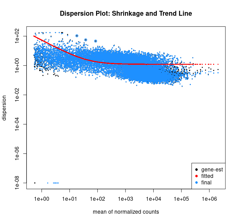
When you look at this plot, you are viewing the visual representation of the "Sharing Information" step:
- Black Dots (MLE): These are the dispersions calculated for each gene individually using only that gene's data. Note how they are very scattered, especially at low counts.
- Red Line (Trend): This is the fit we discussed in Step 2. It represents the "typical" dispersion for a given expression level. If this line doesn't follow the general shape of the black cloud (e.g., it's a flat horizontal line or spikes upward), your data might have serious outliers or batch effects.
- Blue Dots (MAP): These are the final values after Empirical Bayes Shrinkage. They have been pulled from the black dots toward the red line. These are the values actually used for the statistical tests.
- Blue Circles (Outliers): Genes that are extremely variable (far above the trend) are often not shrunk.
DESeq2assumes these have unusually high biological variance and leaves them alone to avoid "over-correcting" true biological signals.
Finally, if you want to extract the actual coefficients of that red line ( and from the equation ), you can find them in the dispersionFunction attribute:
# Extract the trend line function
trend_function <- dispersionFunction(dds)

# View the coefficients
print(attr(trend_function, "coefficients"))
In PyDESeq2, the fitted trend coefficients ($a_0$ and $a_1$ in $\alpha_{tr}(\mu) = a_1/\mu + a_0$) are stored directly on the dataset once fit_dispersion_trend() has run:
# Requires dds.fit_dispersion_trend() to have already been called
print(dds.uns["trend_coeffs"])
Comparison of VST and rlog
We didn't cover rlog in this blog, but the table below can serve as a high-level guide:
| Feature | vst() |
rlog() |
|---|---|---|
| Speed | Fast (Seconds/Minutes) | Slow (Minutes/Hours) |
| Method | Global transformation | Per-gene shrinkage (Bayesian) |
| Best For | Large datasets ($n>30$) | Very small datasets ($n<10$) |
| Requirement | Needs a dispersion trend | Can be sensitive to outliers |
That brings us to the end of this blog. If you're curious to dig deeper into the theory, I highly recommend reading the published research papers I shared above. Hope you find this post useful! 😊